Learn SQL by Calculating Customer Lifetime Value Part 2: GROUP BY and JOIN

This is the second installment of our SQL tutorial blog series. In the first part, we set up the data source with SQLite and learned how to filter and sort data. This time, we will learn two other key concepts in SQL: GROUP BY and JOIN.

GROUP BY: SQL’s Pivot Table

The simplest way to describe GROUP BY is “SQL’s pivot table, except not as powerful.” To explain what I mean by this, let’s review the data from the previous installment.

sqlite> .tables
payments  users

Ah, yes. We had two tables, “users” and “payments.” The “payments” table stored each transaction (let’s say this is data from an e-commerce website), and the “users” table stored what day the user signed up and which campaign source they came from.

sqlite> SELECT * FROM users;
id      	campaign	signed_up_on
----------  ----------  ------------
1       	facebook	2014-10-01
2       	twitter 	2014-10-02
3       	direct  	2014-10-02
4       	facebook	2014-10-03
5       	organic 	2014-10-03
6       	organic 	2014-10-03
7       	organic 	2014-10-04
8       	direct  	2014-10-05
9       	twitter 	2014-10-05
10      	organic 	2014-10-05

sqlite> SELECT * FROM payments;
id      	amount  	paid_on 	user_id
----------  ----------  ----------  ----------
1       	40      	2014-10-02  1
2       	30      	2014-10-03  1
3       	100     	2014-10-04  1
4       	30      	2014-10-05  1
5       	30      	2014-10-06  1
6       	40      	2014-10-07  1
7       	50      	2014-10-08  1
8       	50      	2014-10-09  1
9       	40      	2014-10-10  1
10      	100     	2014-10-11  1

A natural question to ask here is, how much money did each of the 10 users (id=1~10) pay to the website?

If you were using Excel, this is as simple as creating a pivot table:

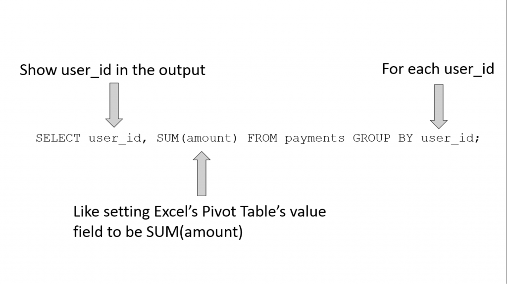
Here is the equivalent operation in SQL, using GROUP BY:

sqlite> SELECT user_id, SUM(amount) FROM payments GROUP BY user_id;
user_id 	SUM(amount)
----------  -----------
1       	1410
2       	1580
3       	35
4       	140
5       	135
6       	1240
7       	105
8       	90
9       	125
10      	105

As the name suggests, the GROUP BY operation groups the table’s rows into different groups based on the column name that follows the “GROUP BY” keyword. In the above query, we have “GROUP BY user_id” so we are grouping the “payments” table based on its “user_id” column.

When you do this, you might get multiple rows in the one group. For example, let’s look at which rows belong to user_id = 1:

sqlite> SELECT * FROM payments WHERE user_id = 1;
id      	amount  	paid_on 	user_id
----------  ----------  ----------  ----------
1       	40      	2014-10-02  1
2       	30      	2014-10-03  1
3       	100     	2014-10-04  1
4       	30      	2014-10-05  1
5       	30      	2014-10-06  1
6       	40      	2014-10-07  1
7       	50      	2014-10-08  1
8       	50      	2014-10-09  1
9       	40      	2014-10-10  1
10      	100     	2014-10-11  1
11      	30      	2014-10-12  1
12      	30      	2014-10-13  1
13      	40      	2014-10-14  1
14      	30      	2014-10-15  1
15      	50      	2014-10-16  1
16      	30      	2014-10-17  1
17      	40      	2014-10-18  1
18      	100     	2014-10-19  1
19      	40      	2014-10-20  1
20      	40      	2014-10-21  1
21      	30      	2014-10-22  1
22      	30      	2014-10-23  1
23      	50      	2014-10-24  1
24      	40      	2014-10-25  1
25      	50      	2014-10-26  1
26      	100     	2014-10-27  1
27      	40      	2014-10-28  1
28      	30      	2014-10-29  1
29      	50      	2014-10-30  1
30      	50      	2014-10-31  1

But here we are not interested in all columns of each group, we are only interested in the “amount” column. More specifically, we are only interested in the sum of the “amount” column per user_id. And this is exactly what “SUM(amount)” does. So, if we were to break the query apart:

Needless to say, GROUP BY can be combined with WHERE (filtering) and ORDER BY (sorting), which are covered in Part 1. Syntactically, WHERE comes before GROUP BY, which in turn comes before ORDER BY.

For example, here is how you can calculate the total for user_id > 5, sorted by the total amount:

sqlite> SELECT user_id, SUM(amount) AS total_amount FROM payments WHERE user_id > 5 GROUP BY user_id ORDER BY total_amount;
user_id     total_amount
----------  ------------
8           90
7           105
10          105
9           125
6           1240

But Where is the Customer Lifetime Value?

At this point, you might be wondering when we are going to discuss customer lifetime value (CLV). In fact, we have already calculated it in the previous section. For our simple model of an e-commerce website, we’ll consider CLV to be the sum of all the purchases a customer has made to date, which is precisely what “SELECT user_id, SUM(amount) FROM payments GROUP BY user_id” does!

So what now?

JOIN: Connecting Multiple Sources of Information

Remember that we began with two tables: “payments” and “users.” We just used the “payments” table to calculate CLV, and previously, we used the “users” table to learn how to use WHERE and ORDER BY.

But also, let’s recall that the “users” table included the “campaign” column indicating which campaign a given user responded to.

Let’s say you wish to determine which campaign (for example, organic/Facebook/Twitter) yields the highest CLV?

If you were using Excel, this is where VLOOKUP comes in. Namely, you VLOOKUP the campaign column in the “users” table in the CLV pivot table that we just computed.
Seeing is believing, so here is a screenshot of what it looks like in Excel:

This is all well and good (I am a big VLOOKUP user myself), but what if you have more than 10 users. What if, say, you have 100,000 users? Excel won’t be able to handle the data, or even if it can, the UI begins to lag. And if you have 10 million users (which happens with decently sized e-commerce websites), Excel is definitely not going to be sufficient.

This is where SQL’s JOIN comes in handy. SQL databases (e.g., MySQL, PostgreSQL, etc.) are far more scalable than Excel – even more so with proper indices – and can perform more complex computations in a more automated manner. (Note: Indexing is a fascinating and deep topic in databases, but it’s beyond the scope of this blog series. Just remember that grouping by indexed columns is much faster than grouping by unindexed columns.) Here is the same operation in SQL. Note that we are first computing the CLV table as before:

sqlite> SELECT cltv.user_id, cltv.cltv, users.campaign FROM (SELECT user_id, SUM(amount) AS cltv FROM payments GROUP BY user_id) cltv JOIN users ON cltv.user_id = users.id;
user_id 	cltv    	campaign
----------  ----------  ----------
1       	1410    	facebook
2       	1580    	twitter
3       	35      	direct
4       	140     	facebook
5       	135     	organic
6       	1240    	organic
7       	105     	organic
8       	90      	direct
9       	125     	twitter
10      	105     	organic

Wow, that’s a lot to unpack, so let me reformat the SQL:

SELECT cltv.user_id, cltv.cltv, users.campaign FROM
  (SELECT user_id, SUM(amount) AS cltv FROM payments GROUP BY user_id) cltv
  JOIN
  users
  ON cltv.user_id = users.id;

The first line chooses columns from the joined table. However, we don’t know how JOINs work yet, so let’s look at the rest of the lines first.

The second line is simply the original CLV calculation. Note that the “SUM(amount)” is aliased as “cltv” as is the resulting “intermediate” table.

The third and fourth lines show that we are joining the “users” table onto the “cltv” table that we just aliased. But how do you join two tables?

This is answered on the last line: it matches the rows of the “cltv” table with the rows of the “users” table so that the “cltv” table’s “user_id” field equals the “users” table’s “id” field. There is no strictly equivalent process for this in VLOOKUP because VLOOKUP forces you to JOIN by the leftmost columns. In SQL, you can JOIN by any desired columns!

The Other CLV: Campaign Lifetime Value

Now that we have a single view of the user IDs, campaign sources and CLVs, we can calculate which campaign has the highest return thus far. To do so, we simply run one more GROUP BY, grouping per-user CLV by campaign:

sqlite> SELECT campaign, SUM(cltv) AS campaign_value FROM (SELECT cltv.user_id, cltv.cltv, users.campaign FROM (SELECT user_id, SUM(amount) AS cltv FROM payments GROUP BY user_id) cltv JOIN users ON cltv.user_id = users.id) GROUP BY campaign;
campaign	campaign_value
----------  --------------
direct  	125
facebook	1550
organic 	1585
twitter 	1705

From this we discover that Twitter is the winner! It looks like there is a healthy amount of organic traffic, comparable to Facebook. Note that this data only accounts for how much revenue is generated for each campaign. Different campaigns have different costs, so if you wish to calculate the ROI of different campaigns (and I hope you do!), you need the data for how much money is spent on each campaign.

Conclusion

• GROUP BY in SQL is like Pivot Table in Excel, except it scales better with larger datasets (especially with proper indices).
• JOIN in SQL is like VLOOKUP in Excel, except JOIN is more flexible.
• You can query against an output of another query to ask more complex questions against your data.

If you want to process massive datasets using SQL, check out Treasure Data, and if you’re interested in use-case specific SQL query templates, check out our library!

Contact me on Twitter @kiyototamura or leave a comment if you have any questions about this.