Dimensionality Reduction Techniques: Where to Begin

When dealing with huge volumes of data, a problem naturally arises. How do you whittle down a dataset of hundreds or even thousands of variables into an optimal model? How do you visualize data through countless dimensions?  Fortunately, a series of techniques called dimensionality reduction aim to help alleviate these issues. These techniques help to identify sets of uncorrelated predictive variables that can be fed into subsequent analyses.

Reducing a high-dimensional data set, i.e. a data set with many predictive variables, to one with fewer dimensions improves conceptualization. Above three dimensions, visualizing the data becomes difficult or impossible. Additionally, reducing dimensions helps to reduce noise by removing irrelevant or highly correlated variables. For analysts working in fields that deal with extreme number of dimensions, like genomics, reducing dimensions will aid in data compression and storage.

There are two main methodologies for reducing dimensions: feature selection and feature extraction. Feature selection centers around finding a subset of the original variables, usually iteratively by finding combinations of subsets and comparing the prediction errors. Feature extraction methods transform the data from high to lower dimensions. Since the data is transformed, it is commonly advised to be cautious of direct interpretations from analyses. For example, in a plot from the t-SNE algorithm, the axes have no meaning in context; they exist only to demonstrate relative distance.

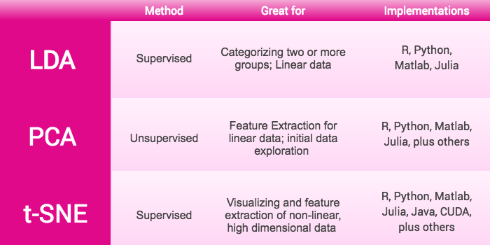
I’ll be focusing on three feature extraction methods: Linear Discriminant Analysis (LDA), Principal Components Analysis (PCA), and t-Distributed Stochastic Neighbor Embedding (t-SNE).

Linear Discriminant Analysis

Linear Discriminant Analysis is a method of dimension reduction that attempts to find a linear combination of variables to categorize or separate two or more groups. While it’s one of the oldest dimensionality reduction techniques, it’s found modern applications in facial recognition and marketing. However, it’s fallen out of favor with techniques like those below being more common. This is because LDA is a supervised learning technique, which requires an analyst to provide a properly defined training set for the analysis to learn on. Errors in the training set propagate in the results, however supervised methods are more accurate . Since LDA is an established technique, it’s been implemented in all major packages: R, Python, Matlab, and Julia.

Principal Components Analysis

Principal Components Analysis (PCA) is one of the most common dimensionality reduction methods and is often a starting point for many analyses. Similar to LDA, Principal Components Analysis works best on linear data, but with the benefit of being an unsupervised method. PCA produces a set of linearly uncorrelated variables called principal components. The first component is determined by its contribution to the greatest variance in the data. Then all subsequent components are found by the same greatest-variability constraint, while also being orthogonal to the previous one. PCA has a close mathematical relationship to other popular methods such as factor analysis and k-Means Clustering. Due to it’s popularity, it’s available in all major packages.

t-Distributed Stochastic Neighbor Embedding

Originally written about in 2008, t-SNE is one of the newest methods of dimensionality reduction. t-SNE differs from the methods listed above in that t-SNE is a non-linear method and performs better on data where the underlying relationship is not linear. This method creates a 2D plane or 3D manifold that preserves the relative distance between observations. This output is then easily visualized as a scatterplot, aiding in visualization. Despite being fairly young compared to LDA and PCA, t-SNE has been openly welcomed in the community since it works exceedingly well where other methods struggle. t-SNE creator Laurens Van Der Maaten gathers the various implementations of t-SNE from across multiple platforms on his github page which is linked below.

Deciding which technique to use comes down to trial-and-error and preference. It’s common to start with a linear technique and move to non-linear techniques when results suggest inadequate fit. Availability of methods widens by having access to a well defined and accurate training set.  Also keep in mind different methods will perform better based on how many dimensions you are trying to reduce by. In order to make a well-informed decision, you may need to experiment and iterate with these different techniques until you find one that works best for your goals and objectives.

For more in depth explanations of each method, see the links below:

• LDA: http://scikit-learn.org/stable/modules/lda_qda.html
• PCA: http://setosa.io/ev/principal-component-analysis/
• t-SNE: https://lvdmaaten.github.io/tsne/ (offers resources, implementations, and FAQ)