Data Science 101: Interactive Analysis with Jupyter, Pandas and Treasure Data
Data Science 101: Interactive Analysis with Jupyter, Pandas and Treasure Data
Data Science 101: Interactive Analysis with Jupyter, Pandas and Treasure Data
In case you were wondering, the next time you overhear a data scientist talking excitedly about “Pandas on Jupyter”, s/he’s not citing the latest 2-bit sci-fi from the orthographically challenged!
Treasure Data gives you a cloud-based analytics infrastructure accessible via SQL. Our interactive engines like Presto give you the power to crunch billions of records with ease. As a data scientist, you’ll still need to learn how to write basic SQL queries, as well as how to use any external tool you choose – like Excel or Tableau – for visualization.
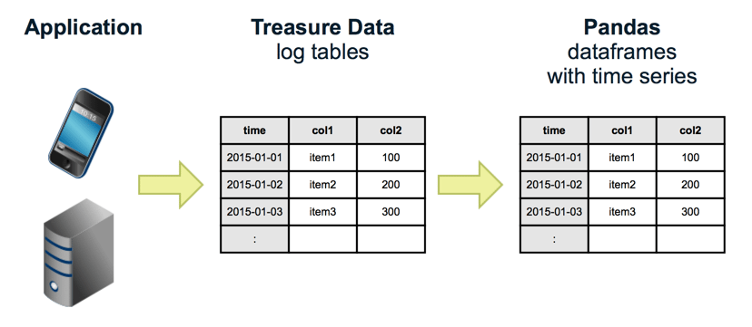
In this article, we’ll show you how to access Treasure Data from the popular Python-based data analysis tool called Pandas, and visualize and manipulate the data interactively via Jupyter (formerly known as the iPython Notebook).
Table of Contents
Prerequisites
Step 0: Set up Treasure Data API key
Step 1: Install Jupyter, Pandas, and Pandas-TD connector
Step 2: Run Jupyter and Create your First Notebook
Step 3: Explore your data
Step 4: Sample your data
See Also
Acknowledgements
Prerequisites
- Basic knowledge of Python
- Basic knowledge of Treasure Data
Step 0: Set up Treasure Data API key
First, set your master api key as an environment variable. Your master API Key can be retrieved from the Console’s profile page.
$ export TD_API_KEY=”5919/abcde…”
Step 1: Install Jupyter, Pandas, and Pandas-TD connector
We recommend that you use Miniconda to install all required packages for Pandas. Download an installer for your OS and install it. Using the package, let’s create a virtual environment for our first project “analysis”. We’ll use Python 3 for this project:
$ conda create -n analysis python=3
…
$ source activate analysis
discarding …/miniconda/bin from PATH
prepending …/miniconda/envs/analysis/bin to PATH
(analysis)$
We need “pandas”, “matplotlib” and “ipython-notebook”:
(analysis)$ conda install pandas
(analysis)$ conda install matplotlib
(analysis)$ conda install ipython-notebook
You can use “pip” for general Python packages. We need “pandas-td”:
(analysis)$ pip install pandas-td
Step 2: Run Jupyter and Create your First Notebook
We’ll use “Jupyter”, formerly known as “IPython notebook” . Run it, and your browser will open:
(analysis)$ ipython notebook
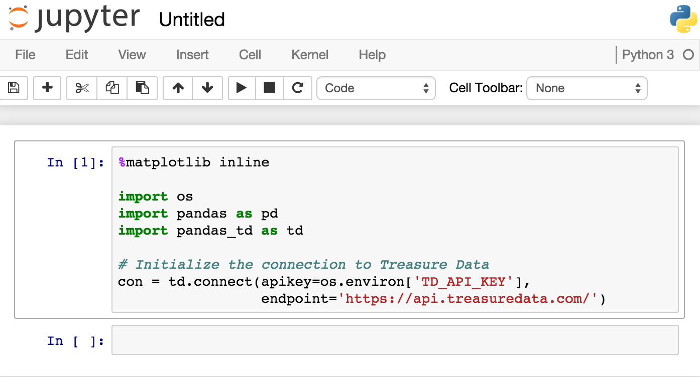
Let’s create a new notebook by selecting from the menus “New . Python 3”. Copy & Paste the following text to your notebook and type “Shift-Enter”:
%matplotlib inline


import os

import pandas as pd

import pandas_td as td


con = td.connect(apikey=os.environ[‘TD_API_KEY’], endpoint=’https://api.treasuredata.com’)
Your notebook now looks something like this:
Step 3: Explore your data
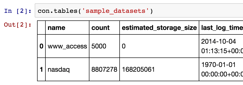
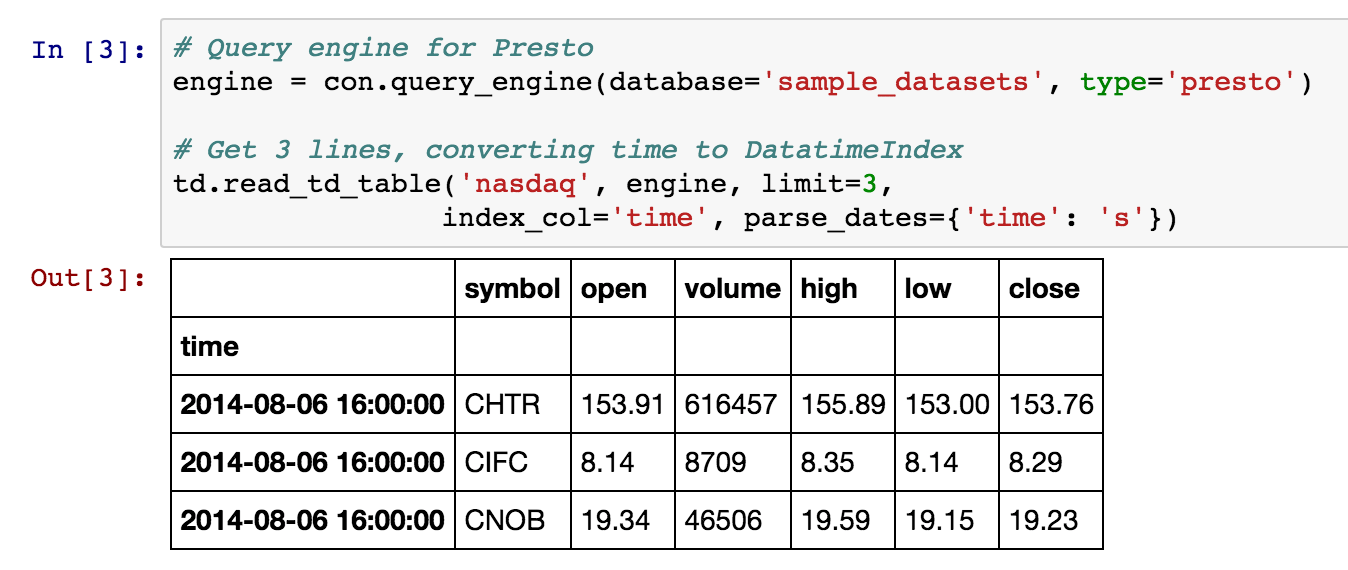
We have two tables in ‘sample_datasets’. Let’s explore the ‘nasdaq’ table as an example.
We’ll use ‘presto’ as a query engine for this session. To see how the table looks, you can retrieve a few lines with the read_td_table function:
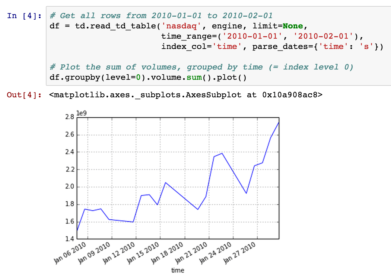
You can also use the time_range parameter to retrieve data within a specific time range:
Now your data is stored in the local variable df as a DataFrame. Since the data is located in the local memory of your computer, you can analyze it interactively using the power of Pandas and Jupyter. For more on that topic, see Time Series / Date functionality.
Step 4: Sample your data
As your data set grows very large, the method from the previous step doesn’t actually scale very well. It isn’t actually a very good idea to retrieve more than a few million rows at a time due to memory limitations or slow network transfer. If you’re analyzing a large amount of data, you need to limit the amount of data getting transferred.
There are two ways to do this:
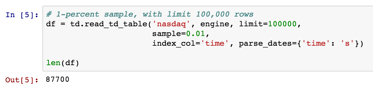
First, you can sample data. We know, for example, that the ‘nasdaq’ table has 8,807,278 rows (at presstime). Sampling 1% of this results in ~88,000 rows, which is a reasonable size to retrieve:
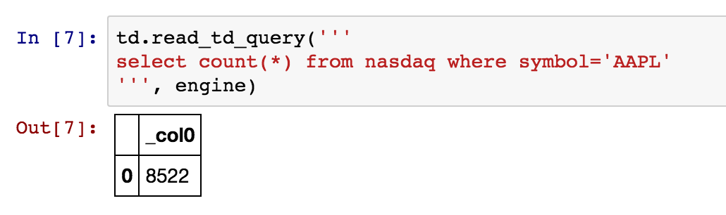
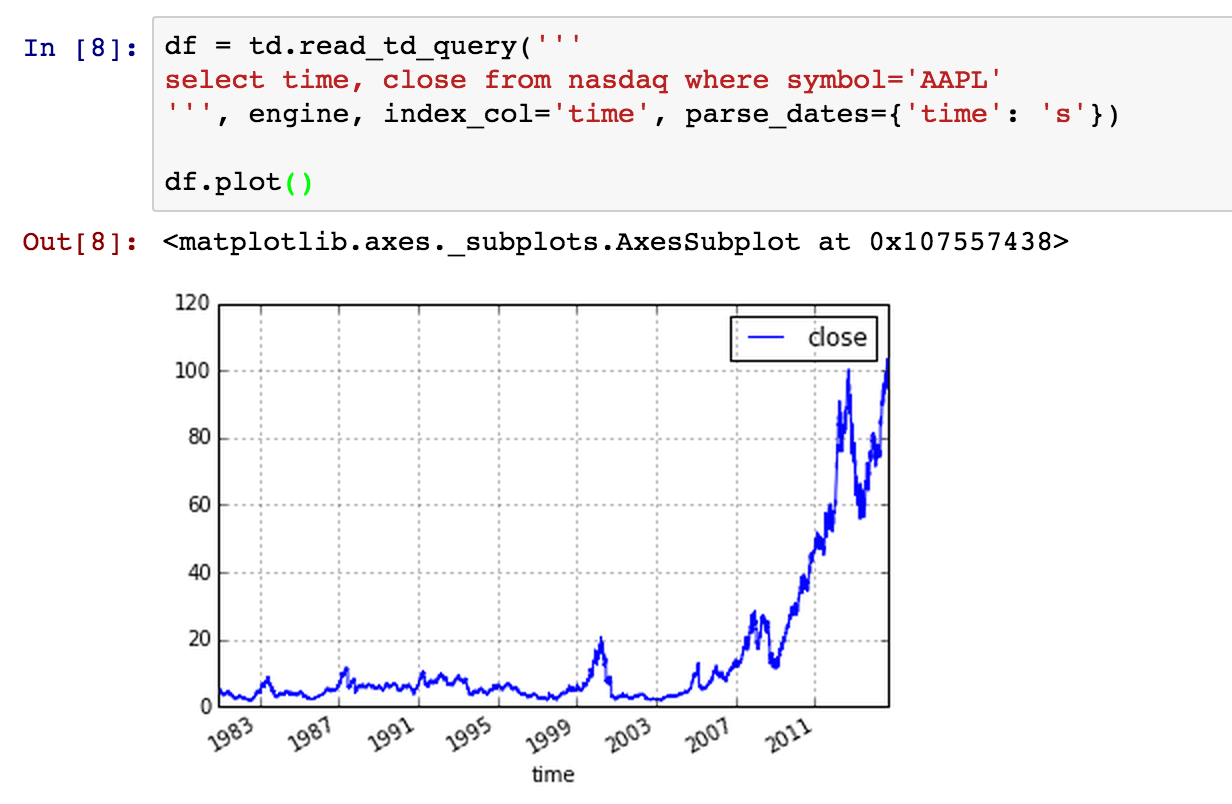
Another way is to write SQL and limit data from the server side. For example, as we are interested only in data related to “AAPL”, let’s count the number of records, using read_td_query:
It’s small enough, so we can retrieve all the rows and start analyzing data:
See Also
- Pandas-TD Github Repository
- Pandas-TD Tutorial
- Python for Data Analysis (Book by Oreilly Media)
- Jupyter Website
- Pandas Website
Note: Jupyter Notebooks are now supported by GitHub and you can share your analysis results with your team.
Acknowledgements
This tool and blogpost are the work of many. A great big thanks goes out to Keisuke Nishida and Kazuki Ohta, among others, for their baseline contributions to – and help on – this article.