Rolling Retention Done Right in SQL
Rolling Retention Done Right in SQL
Rolling Retention Done Right in SQL
SaaS’s Most Important Metric: Retention
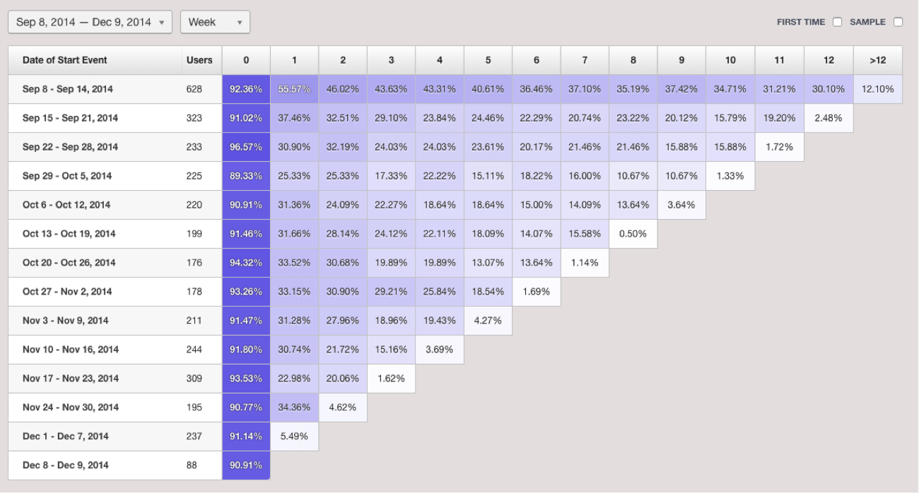
If you are a product manager or in a growth role at a SaaS company, rolling retention (also called cohort analysis) is a key metric to monitor your growth. It’s so important that every analytics service worth their salt (Google Analytics, Mixpanel, Adobe Analytics, Heap Analytics and Amplitude to name few) all have it baked into their UI. Here’s an example from Heap Analytics.
As an organization weans itself off of analytics tools and tries to build their own analytics with SQL and databases, they naturally try to calculate rolling retention using SQL. They soon realize that writing SQL to produce a nice tabular view like the one above isn’t quite straightforward.
But here’s the good news: with a bit of advanced SQL, you can calculate rolling retention against any cohort window with any behavioral condition, assuming that you collect necessary customer events. This is the ultimate reason why you want to use your own database + SQL v. canned analytics tools: the infinite flexibility in defining, tweaking and improving your retention analysis to drive growth.
Rolling Retention: Definition
Before we dive into SQL, here’s a quick review of rolling retention, also known as cohort analysis.
Rolling retention is defined as the percentage of returning users measure at a regular interval, typical weekly or monthly, grouped by their sign-up week/month, also known as cohort. By grouping users based on when they signed up, you can gain insight on how your product/marketing/sales initiatives have impacted retention: For example, suppose you had a major launch and had many sign-ups over the following few days. How well did these new users stick around compared to, say, pre-launch users that signed up a week prior? Or, say you sent out offers for a discount to dormant users from 2 months ago: How many of them came back and stayed on the product? Rolling retention helps you answer these questions at a glance.
Setting the Stage
In the rest of this article, we assume that you have a table called “logins” with just two columns: user_id and login_time. Here’s an example:
| user_id | login_time |
|---|---|
| a005baae | 1468571605 |
| a005baae | 1468571605 |
| a03224fb | 1468571605 |
| a03224fb | 1468571605 |
| a03224fb | 1468571605 |
| a05e88ec | 1468598437 |
| a05e88ec | 1468615063 |
| a05e9452 | 1468569072 |
Note that we are using Unix (epoch) time for the time field, which indicates the number of seconds since Jan 1, 1970 UTC. The decision to use Unix time is a conscious one. Because Unix time is of an integer type and has a clear meaning, we can focus on the core logic and avoid reasoning about time zones and other tangential issues.
Also, I will be working with weekly cohorts. Depending on your product/internal process, you might want to adjust it to daily or monthly.
Finally, in the rest of this article, I am using Treasure Data’s flavor of Presto SQL. That said, the core logic should work on any SQL engine.
Step 1: Bucketing Visits By Week
The first step is to bucket visits into cohorts, i.e., which user loggedin into the app at all in a given week. To do this, we are grouping users by week as follows:
The query “squashes” all logins in each week into one row for each user. “TD_DATE_TRUNC” function is used to do this. Also, note that Presto SQL lets you alias column names in the GROUP BY clause with their ordinals.
Step 2: Normalizing Visits
The next step is to calculate the number of weeks between the week of the first visit and the given visits’ week. Said another way, give the following table:
| user_id | login_week |
|---|---|
| a005baae | 1462147200 |
| a005baae | 1462752000 |
| a03224fb | 1462147200 |
| a03224fb | 1462752000 |
| a03224fb | 1463356800 |
| a05e88ec | 1462752000 |
| a05e88ec | 1463356800 |
| a05e9452 | 1462752000 |
You create the “first_week” and “week_number” columns.
| user_id | login_week | first_week | week_number |
|---|---|---|---|
| a005baae | 1462147200 | 1462147200 | 0 |
| a005baae | 1462752000 | 1462147200 | 1 |
| a03224fb | 1462147200 | 1462147200 | 0 |
| a03224fb | 1462752000 | 1462147200 | 1 |
| a03224fb | 1463356800 | 1462147200 | 2 |
| a05e88ec | 1462752000 | 1462752000 | 0 |
| a05e88ec | 1463356800 | 1462752000 | 1 |
| a05e9452 | 1462752000 | 1462752000 | 0 |
So, how do you do this?
The answer is to use the FIRST_VALUE window function.
First, note that we “saved” the previous query using the “WITH” query into the temporary table by_week.
Second, note how FIRST_VALUE is used. The mechanics of window functions is a whole topic to itself, but in this case, it partitions login_time by user_id, order them in ascending order by itself, and get the first value. Hence, the result of the query is:
| user_id | login_week | first_week |
|---|---|---|
| a005baae | 1462147200 | 1462147200 |
| a005baae | 1462752000 | 1462147200 |
| a03224fb | 1462147200 | 1462147200 |
| a03224fb | 1462752000 | 1462147200 |
| a03224fb | 1463356800 | 1462147200 |
| a05e88ec | 1462752000 | 1462752000 |
| a05e88ec | 1463356800 | 1462752000 |
| a05e9452 | 1462752000 | 1462752000 |
From here, it’s easy to calculate week_number by subtracting login_week from first_week and dividing by 24*60*60*7 (recall that Unix time is in seconds). Hence, the final query is:
And You are done calculating week_number. Phew!
Step 3: Tallying Up
We are almost done. Now, we need to create the “pivot table” view of retention analysis. In general, most SQL engines don’t support the full pivot table functionality with dynamic columns. In our case, however, we can mimic it with the SUM function and the CASE statement because we only need to compute number of visitors for week 0 through 9 per cohort.
Here is the actually query:
Which yields:
| first_week | week_0 | week_1 | week_2 | … |
|---|---|---|---|---|
| 5/1/16 | 2 | 2 | 1 | … |
| 5/8/16 | 2 | 1 | 0 | … |
This gives you the raw user counts for each cohort week over week. If you want to convert the columns into percentage, then divide week_1 through week_9 with week_0.
Why Do This?
If you aren’t a SQL veteran, you might have found the above queries a bit daunting. Why go through so much trouble if these cohort reports are already available in analytics tools?
Because SQL is more expressive, customizable and powerful.
Here are some known limitations that I’ve personally run into with canned analytics tools for retention analysis:
- Adjusting conversion windows: Many tools have a fixed/limited set of conversion windows for funnel analysis, such as “up to 180 days” or “30, 60 or 90 days”. However, the sales cycle varies from one SaaS to another, and it’s helpful to have the flexibility to adjust the conversion window.
- Defining custom conversion events: To be sure, analytics services do let you customize events. That said, these custom events often require explicit definitions and/or cannot be modified post facto. By collecting raw events and analyzing them in SQL, you gain full flexibility in defining and evolving your conversion events.
- Combining with Salesforce data to filter “bad” conversions: Not all sign-ups are created equal; some are tire-kickers, while others can turn into a multi-million dollar account. Unfortunately, these types of account/lead-level information are not captured in analytics tools, but rather in CRM tools like Salesforce or customer support tools like Zendesk. Thanks to Treasure Data’s Salesforce and Zendesk data connectors, you can bring customer metadata into your retention analysis. And it allows you to calculate deeper metrics, such as revenue retention or retention by geography or buyer persona.
If you are curious to learn how Treasure Data can take your customer analytics to the next level, read how our customers are using our service or request a product demo below.