Accurate Sales Forecast for Data Analysts: Building a Random Forest model with Just SQL and Hivemall
Accurate Sales Forecast for Data Analysts: Building a Random Forest model with Just SQL and Hivemall
Accurate Sales Forecast for Data Analysts: Building a Random Forest model with Just SQL and Hivemall
In this blog post, we will use Hivemall, the open source Machine Learning-on-SQL library available in the Treasure Data environment, to introduce the basics of machine learning. We will use an E-Commerce dataset from Kaggle, the data science competition platform.
Introduction
The first challenge is predicting the retail sales for the Rossman stores (the full details at Kaggle). We will use an ensemble learning technique known as Random Forest regression.
Rossman is a pharmacy chain with over 3,000 stores in seven countries within Europe. The manager of each store has been tasked to predict the sales of the store for up to six weeks in advance. Sales of each store depends on various factors such as each store’s promotional activities, public and school holidays, seasonal and regional characteristics.
For the competition, Rossmann has provided training data for each day in 1,115 of their stores over six weeks in Germany from January 1, 2013 to July 31, 2015. The test data set runs from August 1, 2015 to September 17, 2015.
Next we will explain in detail how to analyze this data on Treasure Data using Hivemall.
Preparing the Data
Importing into Treasure Data
Rossman Store Sales task provides three datasets in CSV format: the training data set (train.csv), the verification data set (test.csv) and the store information data set. Stores are identified by Store IDs in all three datasets.
After downloading the data from Kaggle, you can drag-and-drop the files into Treasure Data through the File Upload option. Treasure Data automatically creates the table definition by looking at the header as well as the actual data columns.
Each data file is configured as follows:
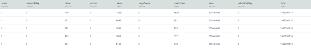
Training Data (train.csv)
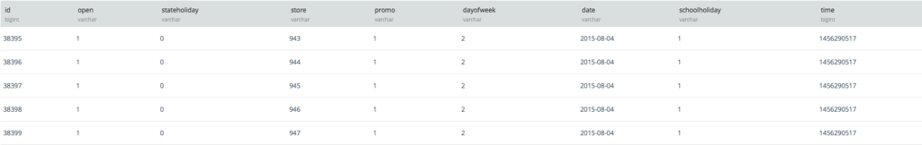
Testing Data (test.csv)
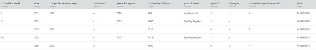
Store Information (store.csv)
With data information described below:
| Column Name | Type | Description |
|---|---|---|
| ID | Unique Identifier | An ID that represents a store and date duple within the test set |
| Sales | Response Variable / Continuous | the sales for one day for that shop (This is what you are predicting) |
| Store | Categorical | Unique ID assigned to each shop |
| Customers | Continuous | The number of customers visiting that store in one day |
| Open | Categorical | 0 if store is closed that day, 1 if open |
| StateHoliday | Categorical | Indicates a state holiday. Normally stores are closed on a holiday: a = public holiday, b = Easter holiday, c = christmas, 0 = None |
| SchoolHoliday | Categorical | Indicates if the store was affected by the closure of public schools on that date |
| StoreType | Categorical | Defines which of four different store models the store is: a, b, c, d |
| Assortment | Categorical | Describes the item assortment level: a = basic, b = extra, c = extended |
| CompetitionDistance | Categorical | The distance in meters to the nearest competitor store |
| CompetitionOpenSince [Month / Year] | Categorical | Gives the approximate year and month that the nearest competitor was opened |
| Promo | Categorical | Indicates where a store is running a promotion that date |
| Promo2 | Categorical | Promo2 is a continuing and consecutive promotion for some stores: 0 = store is not participating, 1 = store is participating |
| Promo2Since [Year / Week] | Categorical | Describes the year and calendar week when the store started participating in Promo2 |
| PromoInterval | Categorical | Describes the consecutive intervals Promo2 is started, naming the months the promotions is started anew. E.g. “Feb,May,Aug,Nov” means each round starts in February, May, August, November of any given year for that store |
Visualizing the Data
Let’s take a look at the sales data for Store ID = 1. This script visualizes the data using the TD-pandas package and Jupyter Notebook.
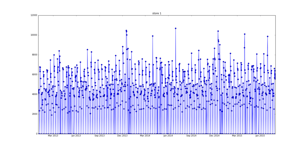
By visualizing the data, we are able to review both the cyclic patterns of the amount of sales as well as the spikes in the data.
Visualization helps us infer what features (the day of week, weekend/weekdays, etc.) can be used to account for periodicity.
Pre-processing the Data
Joining the Data
First, we want to join the store information in the training set (including information such as the promotions and competing stores.
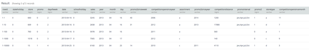
It should be noted that the date is a string in the format of yyyy-mm-dd (such as, for example, 2014-05-25), so we will need to extract year, month, and day as partial strings. Additionally, we excluded from the training any rows where sales were equal to zero that day.
The results of the above Hive query are stored in training2 and shown below.
Generating the Feature Vector
The table, training2, that we created in the previous step, contains non-numeric data. In this step, we will convert the non-numeric data to numeric data so that we can create a feature vector that can be fed into the Random Forest algorithm. A feature vector is an array that represents each feature quantity as a numerical value.
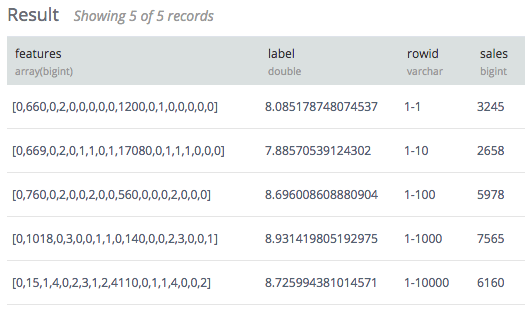
The quantify function seen here converts the non-numeric columns to numeric by outputting a numeric ID. In addition, missing values are replaced with zeroes and the response variable, sales, is transformed using a log scale conversion.
The converted table is as follows:
Preparing the Testing Data
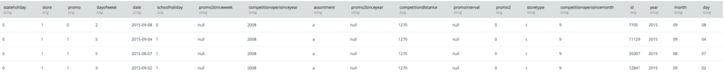
We also need to transform the test data by joining the store information table with the testing data.
The resulting table is shown below:
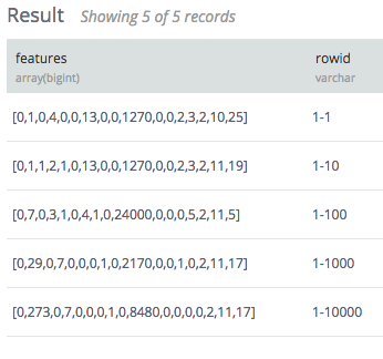
Next, it is necessary to make the same conversion of categorical to continuous variables that we did earlier in the training data, and then process the test data. For example, StoreType can be either a, b, or c but there is also a fourth type d, in the training data. If we mapped categorical variables separately for the training and the test data sets, there would be a mismatch later. The above transformation accounts for this case.
The results of the final test tables is as follows:
Using Random Forest
Now with the training data we created in the last step, we can finally apply the Random Forest algorithm. Random Forest is an ensemble learning technique that constructs multiple decision trees via randomization. In this analysis, we will build 100 different trees.
The query below runs the algorithm. Here, we create the 100 trees by running 5 parallel regressions that create 20 trees each and then using UNION ALL to bring them together. The ‘-Attrs’ flag defines what variables are categorical and which are continuous, with variables with the option C being categorical and those with an option Q being continuous. Only the column competition distance is a continuous variable.
Selecting Variable Importance
From the results of the Random Forest query, we can show how much each explanatory variable affects the model. Using a combination of Jupyter notebook, Pandas and some visualization, we can see the execution results as a bar chart.
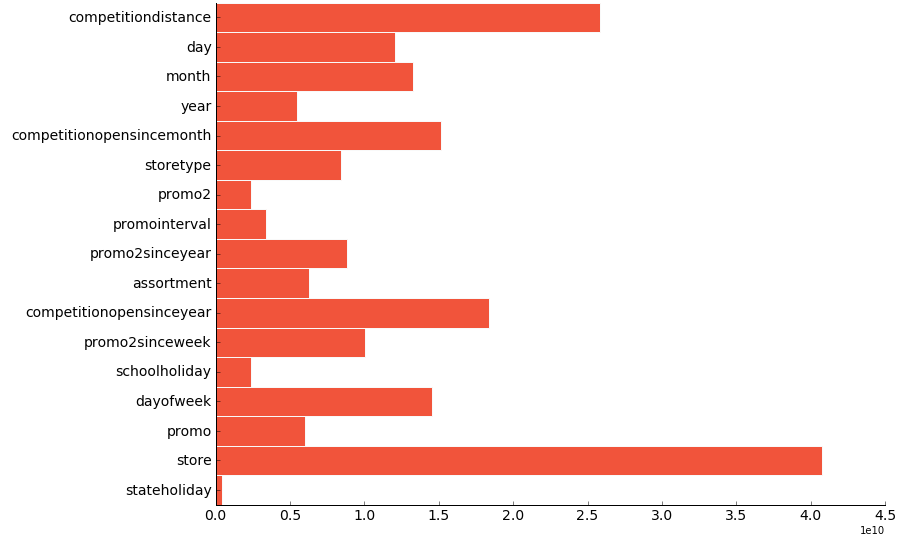
The bar chart suggests that which store it is and the distance to its nearest competition affects the of the store the most. This is consistent with the intuition that stores themselves have a big influence on its sales numbers, and if there’s a competitor nearby, they can eat into your sales.
The Jupyter notebook that generated the visualization can be seen below.
Prediction
Next we’ll make a prediction using the model we created. The response variable at the time of learning is LN(1 + t1.sales) after converting the scale, so the reverse conversion would be EXP(predicted-1).
To submit the results to Kaggle, we’ll sort the prediction results in ascending order of Store ID.
Evaluation
To evaluate the strength of our predictions, we will use the following equation:
Where yi is the sales of that the ith day for that store, and y^i is the predicted value.
The code use to cross-validate can be found here.
Conclusion
Kaggle is the perfect place to learn the basics of data analysis. The sales prediction analysis shown today could be applied to various applications, like e-commerce or advertising campaigns.
Treasure Data provides a flexible and turn-key environment to upload, pre-process and train data sets for machine learning. If you are interested in learning more, please follow the link below to request a demo.